5 Aerodynamics

Recurring Terminology

Symbol	Definition
$a$	slope of lift curve, $dC_L/d\alpha$
$\mathrm{ac}$	aerodynamic center, location along the chord where pitching moments about this center do not change with angle of attack (25% $\mathrm{MAC}$ for airfoils in subsonic flow, 50% $\mathrm{MAC}$ for airfoils in supersonic flow)
$\mathrm{AOA}$	angle of attack
$\mathrm{AR}$	aspect ratio $= [\text{wing span}]^2 / [\text{reference wing area}] = b^2/S$
$B$	wing span
$b_t$	horizontal tail span
$C$	coefficient, a non-dimensional representation of an aerodynamic property
$c$	wing chord length Camber maximum curvature of an airfoil, measured at maximum distance between chord line and amber line, expressed in % of $\mathrm{MAC}$. Camber line theoretical line extending from an airfoil’s leading edge to the trailing edge, located halfway between the upper and lower surfaces.
$C_D$	drag coefficient
$C_{D_i}$	induced drag coefficient
$C_{D_0}\text{, }C_{D_{\mathrm{PE}}}$	parasitic drag coefficient
$c_f$	friction coefficient
Chord	straight-line distance from an airfoil’s leading edge to its trailing edge
$C_L$	lift coefficient
$C_p$	pressure coefficient = $\Delta p/q$
$e$	Oswald efficiency factor
$l$	distance traveled by flow, or characteristic length of surface
$M$	Mach number
$\mathrm{MAC}$	mean aerodynamic chord, chord length of location on wing where total aerodynamic forces can be concentrated.
$\mathrm{MGC}$	mean geometric chord, the average chord length, derived only from a plan form view of a wing (similar to $\mathrm{MAC}$ if wing has no twist and constant cross section & thickness-to-chord ratio).
$P$	pressure
$P_\text{req'd}$	power required
$q$	dynamic pressure = $\frac{1}{2} \rho_a V_T^2 = \frac{1}{2} \rho_0 V_T^2$
$R$	gas constant
$\mathrm{Rn},\mathrm{Re}$	Reynolds number
$S$	reference wing area, includes extension of wing to fuselage centerline.
$S_t$	horizontal tail surface area
$S_W$	wetted area of surface
$T$	temperature
$V$	true velocity
$V_e$	equivalent velocity
$\alpha$	angle of attack
$\alpha_i$	induced angle of attack
$\delta$	depth of boundary layer, or surface wedge angle
$\mu$	viscosity, or wave angle
$\nu$	flow turning angle
$\theta$	shock wave angle
$\rho$	density

• Perfect Fluid
  • incompressible, inelastic, and non-viscous
  • used in flow outside of boundary layers at $M$ < .7
• Incompressible, inelastic, viscous
  • used for boundary layer studies at $M$ < .7
• Compressible, non-viscous, elastic fluid
  • used outside boundary layers up to $M$ = 5

5.1 Dimensional Analysis Interpretations

(ref 5.2)

Aerodynamic force = $F$

• $F = f \left( \rho \text{, } \mu, T \text{, } V \text{, shape, orientation, size, roughness, gravity} \right)$
• For aircraft ignore $R$, $K$ & hypersonic effects

• Initially assume similar body orientations, shapes & roughness.
• Dimensional Analysis reveals four non-dimensional ($\pi$) parameters:
  • Force Coefficient $\pi_1 = \frac{F}{\rho V^2 l^2}$
  • Reynolds Number $\pi_2 = \frac{\rho V l}{\mu}$
  • Mach Number $\pi_3 = \frac{V}{a}$
  • Froude Number $\pi_4 = \frac{V}{\sqrt{lg}}$

A closer look at the force coefficient:

$$C_F = \frac{F}{\rho V^2 l^2} => \frac{F}{\frac{1}{2} \rho V^2 S}$$

where $\frac{1}{2} \rho_a V_T^2 = \frac{1}{2} \rho_0 V_e^2 = \text{dynamic pressure}\text{, }q$

Dimensions of reference wing area, $S$ are the same

A feel for $q$

• Kinetic energy of a moving object = $\frac{1}{2} m V_T^2$
• Block of moving air kinetic energy = $\frac{1}{2} \rho \text{ (volume) } V_T^2$
• Dividing through by volume yields $\mathrm{KE}$ per volume of moving air = $\frac{1}{2} \rho V_T^2$
• “Dynamic pressure” or “$q$” = potential for converting each cubic foot of the airflow’s kinetic energy into frontal stagnation pressure
• Feel $q$ by extending your hand out the window of a moving car

A feel for coefficients

• $C_F = (F/S)/q$ = the ratio between the total force pressure and the flow’s dynamic pressure
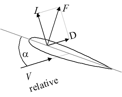
• Lift is the component of the total force perpendicular to the free stream flow
• Drag is the component along the flow
• Break total into lift and drag coefficients:
  • $C_L = (L/S)/q$
  • $C_D = (D/S)/q$
• Increasing dynamic pressure generates a larger total force, lift and drag

• Froude number is not significant in aerodynamic phenomena
• Recall that forces are also a function of angle of attack, shape & surface roughness, therefore

$$C_L,C_D = f \left[ M \text{, } \mathrm{Re} \text{, } \alpha \right] \text{ for a given shape, roughness}$$

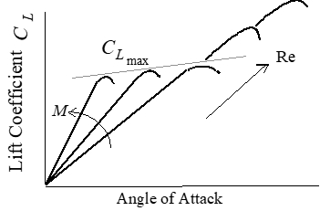
Note in the figure above the Reynolds effects are exaggerated

To compare test day and standard day aircraft or to match wind tunnel $C_F$ data to actual aircraft; the shape, roughness, $M$, $\mathrm{Rn}$ and $\alpha$ must be equal for both aircraft

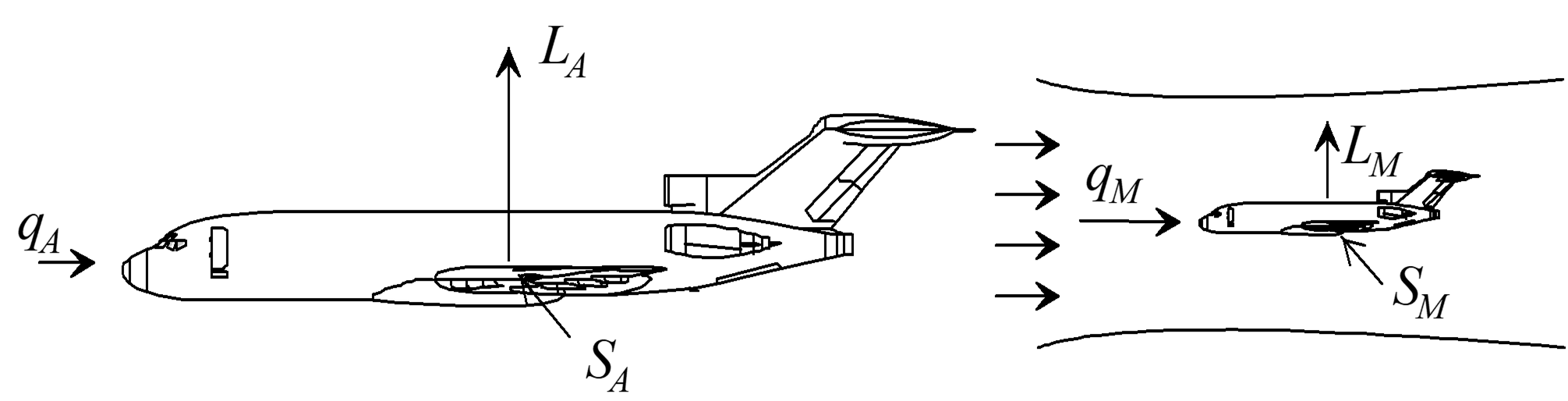
$$\frac{L_A}{q_A S_A} = C_L = \frac{L_M}{q_M S_M}$$

5.2 General Aerodynamic Relations

(refs 5.1, 5.2, 5.10)

Lift & Drag forces can be described using two approaches:

1. Change in momentum of airstream, $F=d[mv]/dt$
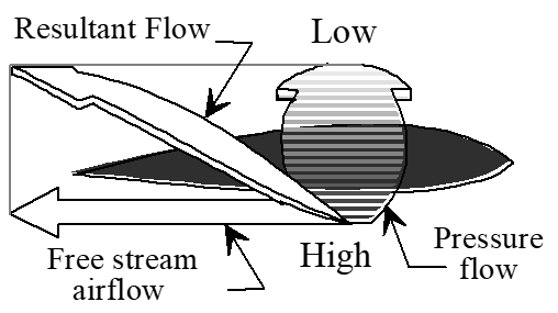
2. “Bernoulli” approach which requires the continuity and conservation of energy equations

Continuity Equation

Fluid Mass in = Fluid Mass out

$$\rho_1 V_1 A_1 = \rho_2 V_2 A_2$$

For subsonic (incompressible) flow $\rho_1 = \rho_2$

$$V_1 A_1 = V_2 A_2$$

Conservation of Energy (Bernoulli) Equation:

Potential + Kinetic + Pressure = constant (changes in Potential energy are negligible)

Energy per unit volume is pressure then Dynamic Pressure + Static Pressure = Total Pressure

$$\frac{1}{2}\rho V^2 + p_s = \text{constant}$$ $$\frac{1}{2}\rho V^2 + p_s = p_t$$

• This classic approach only applies in the “potential flow” region and not in the boundary layer where energy losses occur
• Pressures around a surface can be calculated or measured from tests and converted into pressure coefficients,

$$c_p = \left( p_{\mathrm{local}} - p_{\mathrm{ambient}} \right) / \text{dynamic pressure} = \Delta p/q$$

• $c_p$ values can be mapped out for all surfaces

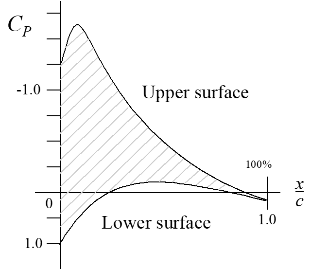
• Summation of all pressures perpendicular to surface yield the pitching moments and the “Resultant Aerodynamic Force” which is broken into lift and drag components

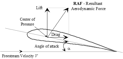
• Lift & drag forces are referred to the aerodynamic center ($\mathrm{ac}$) where the pitching moment is constant for reasonable angles of attack.
• Pitching moments increase with airfoil camber, are zero if symmetric.
• Aerodynamic center is located at 25% $\mathrm{MAC}$ for fully subsonic flow and at 50% $\mathrm{MAC}$ for fully supersonic flow.

5.3 Wing Design Effects on Lift Curve Slope

(refs 5.1, 5.2, 5.10)

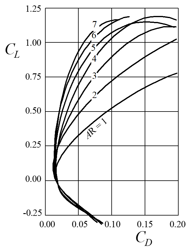
Aspect Ratio Effect

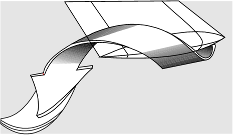
• Pressure differential at wingtip causes tip vortex

• Vortex creates flow field that reduces $\mathrm{AOA}$ across wingspan

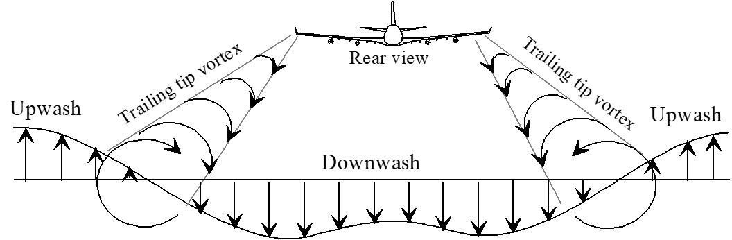
• Local $\mathrm{AOA}$ reductions decrease average lift curve slope

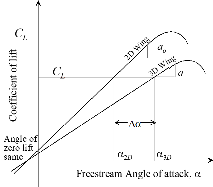
2D wing = wind tunnel airfoil extending to walls (infinite aspect ratio).

$a_0 = \text{Lift curve slope for an infinite wing}$

$a = \text{Lift curve slope for a finite wing}$

• Above relationship estimated as $\alpha = \frac{dC_L}{d \alpha} = \frac{a_0}{1+\frac{57.3 a_0}{\pi \mathrm{AR}}}$

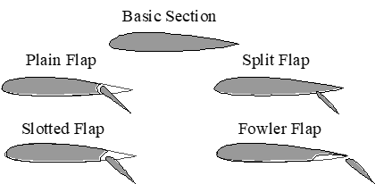
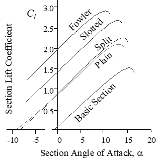
Trailing Edge Flap Effects

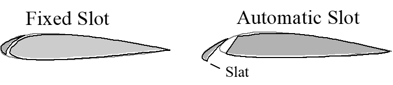
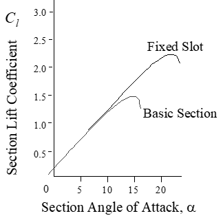
Leading Edge Flap Effects

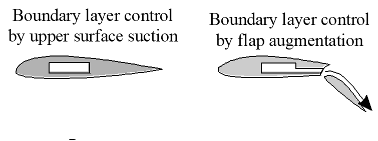
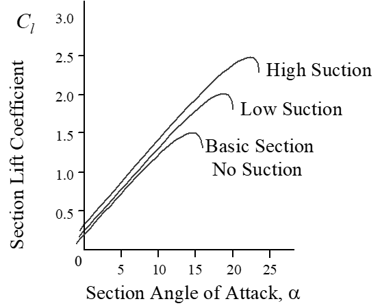
Boundary Layer Control Effects

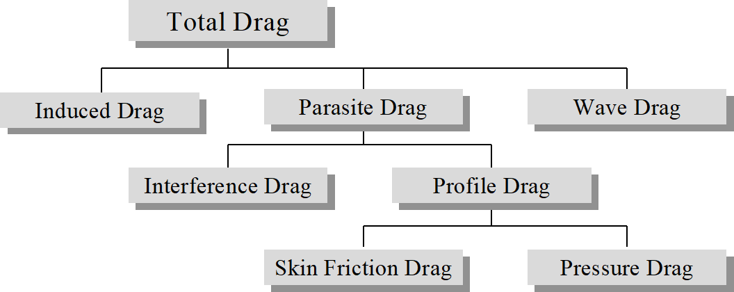
5.4 Elements of Drag

(refs 5.1, 5.2, 5.10)

• Skin friction shear stress is a function of velocity profile at surface

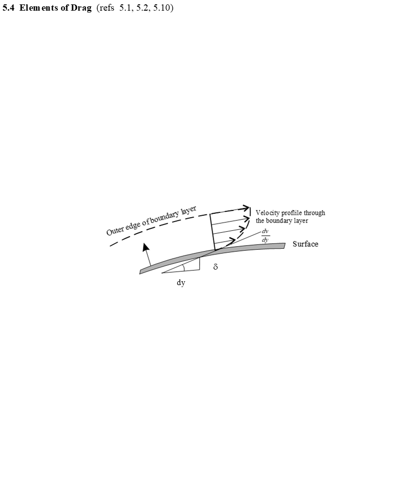
Shear stress $\tau_w = \mu \left( \frac{dv}{dy} \right)_{y=0}$

• Viscosity $\mu$ increases with temperature (ref 5.9)

Sutherland law: $\mu = \mu_0 \frac{\left( \frac{T}{T_0} \right)^{1.5} \left( T_0 + S \right)}{\left( T + S \right)}$

Power law: $\mu = \mu_0 \left( \frac{T}{T_0} \right)^n$

Where $T_0 = 273.15 \text{K} = 518.67 \text{R}$

For air: $S = 110.4 \text{K} = 199 \text{R} \text{; n=0.67}$

For air at $273$ K : $\mu_0 = 1.717 \times 10^{-5} \left[\text{kg/m s}\right] = 3.59 \times 10^{-7} \left[\text{slug/ft s}\right]$

Inserting air values ($T_K=$Kelvin and $T_R=$Rankin) into Sutherland law gives

$$\mu = 1.458 \times 10^{-6} \frac{T_K^{1.5}}{T_K+110.4} \left[\frac{\text{kg}}{\text{s m}}\right] = 2.2 \times 10^{-8} \frac{T_R^{1.5}}{T_R+199} \left[\frac{\text{slug}}{\text{s ft}}\right]$$

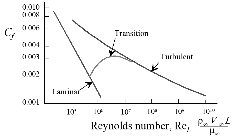
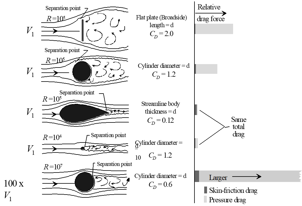
5.4.1 Reynolds Number Effects

(ref 5.10)

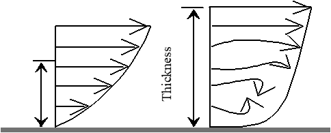
• Laminar boundary layers have more gradual change in velocity near surface than turbulent boundary layers.
• High Reynolds numbers help propagate turbulent flow.

Shearing stress: $\tau_w = \mu \left(\frac{dv}{dy}\right)_{y=0}$

Skin friction coefficient: $C_f = \frac{\tau_w}{\frac{1}{2}\rho_{\infty} V_{\infty}^2} = \frac{\tau_w}{q_{\infty}}$

Laminar boundary layer: $\text{Total } C_f = \frac{1.328}{\left(\mathrm{Re}_L \right)^{1/2}}$

Turbulent boundary layer: $\text{Total } C_f = \frac{0.455}{\left(\log(\mathrm{Re}_L)\right)^{2.58}} \approx \frac{0.074}{\left(\mathrm{Re}_L\right)^{1/5}}$

$\mathrm{Re}_L$ based on total length of flat plate

• Depth of boundary layer $(\delta)$ depends on local Reynolds number $(\mathrm{Re}_x)$ and whether the flow is turbulent or laminar.

$$\mathrm{Re}_x = \frac{\rho_{\infty} V_{\infty} x}{\mu_{\infty}} \equiv \frac{\text{Inertia Forces}}{\text{Viscous Forces}}$$

$x =$ distance traveled to point in question

$$\delta_{\mathrm{lam}} = \frac{5.2x}{\sqrt{\mathrm{Re}_x}}$$

$$\delta_{\mathrm{turb}} = \frac{0.37x}{\mathrm{Re}_x^{0.2}}$$

5.4.2 Pressure Drag

• Ideal frictionless flow has no losses and leads to zero pressure drag
• Real fluids have friction and energy losses along surface
• Energy losses negate total pressure recovery, lead to decreasing total pressure along surface

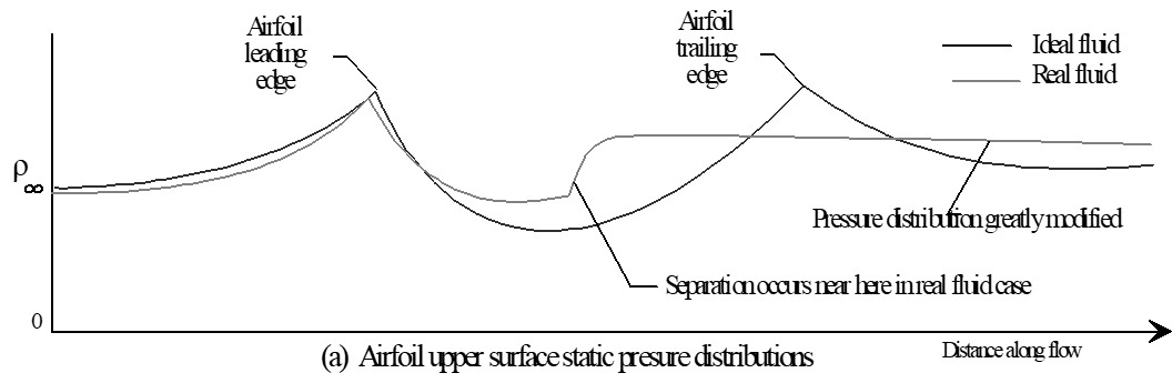
• Imbalance of pressures on surfaces causes pressure drag

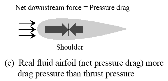
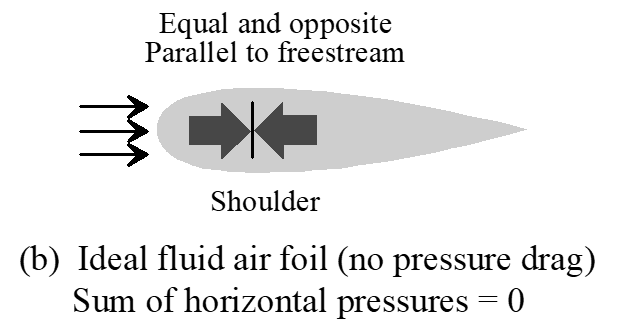
• Profile streamlining reduces pressure drag

5.4.3 Interference Drag

• Occurs with multiple surfaces approximately parallel to flow
• Caused by flow’s interference with itself or by excessive adverse pressure gradient due to rapidly decreasing vehicle cross section
• Most severe with surfaces at acute angles to each other
• Effects often reduced by fillets around contracting surfaces

5.4.4 Induced Drag

• Wingtip vortex reduces local $\mathrm{AOA}$ at each station along wing
• Local lift vector is perpendicular to local $\mathrm{AOA}$
• Local lift vector is therefore tilted back relative to freestream lift
• Induced drag defined as rearward component of local lift vector

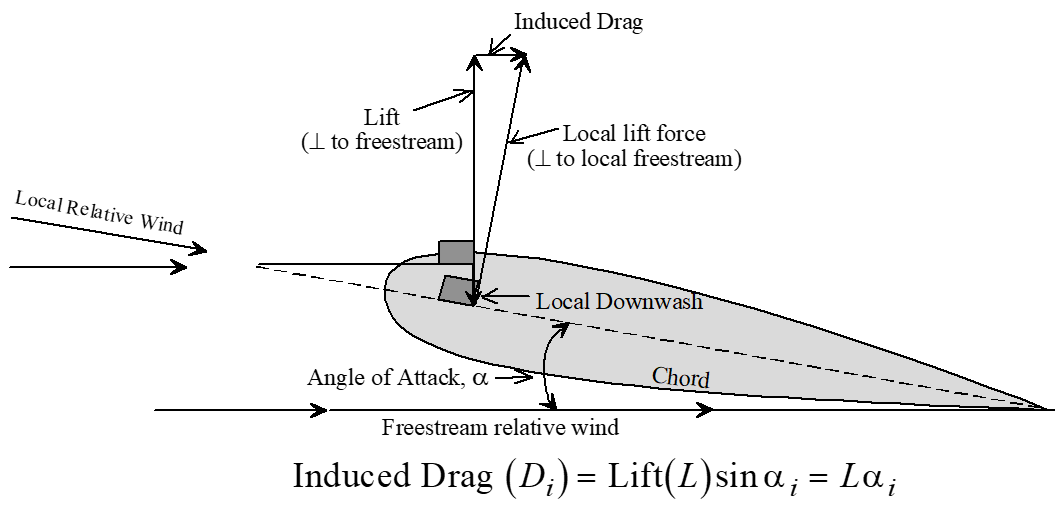
Induced Drag $$\left(D_i\right)=L\left(\alpha_i\right)$$

For elliptical lift distributions $\alpha_i = \frac{C_L}{\pi \mathrm{AR}}$

$$\therefore D_i = L \left(\frac{C_L}{\pi \mathrm{AR}}\right) \text{ but } L=qSC_L$$

$$C_{D_i} = \frac{D_i}{qS} = \frac{C_L^2}{\pi \mathrm{AR}}$$

Oswald efficiency factor, $e$, accounts for losses in excess of those predicted above (due to uneven downwash and changing interference drag effects).

$$\therefore C_{D_i} = \frac{C_L^2}{\pi \mathrm{AR} e}$$

5.5 Aerodynamic Compressibility Relations

(ref 5.8)

Prandtl/Glauert Approximation

Approximates Mach effects on aerodynamics below critical Mach

$$C_{P_{\mathrm{compressible}}} = \frac{1}{\sqrt{1-M^2}}C_{P_{\mathrm{incompressible}}}$$

Total vs Ambient Property Relations for Adiabatic Flow

$$\frac{T_T}{T} = 1 + \frac{\gamma -1}{2}M^2 \text{ Isentropic flow not required}$$ $$\frac{P_T}{P} = \left[1 + \frac{\gamma - 1}{2}M^2 \right]^{\frac{\gamma}{\gamma-1}} \text{ Isentropic (shockless) flow required}$$ $$\frac{\rho_T}{\rho} = \left[1 + \frac{\gamma - 1}{2} M^2 \right]^{\frac{1}{\gamma -1}} \text{ Isentropic flow required}$$

Normal Shock Relations

Assumes isentropic flow on each side of the shock Assumes flow across shock is adiabatic Property changes occur in a constant area (throat)

$$\frac{P_2}{P_1} = \frac{1 - \gamma + 2\gamma M_1^2}{1+\gamma}$$ $$\frac{\rho_2}{\rho_1} = \left[\frac{2 + \left(\gamma - 1\right) M_1^2}{\left(\gamma+1\right) M_1^2} \right]^{-1}$$ $$\frac{T_2}{T_1} = \left[\frac{1 - \gamma + 2\gamma M_1^2}{1 + \gamma} \right]\left[\frac{2 + \left(\gamma - 1\right) M_1^2}{\left(1 + \gamma\right) M_1^2} \right]$$ $$M_2^2 = \frac{M_1^2 + \frac{2}{\gamma - 1}}{\frac{2\gamma}{\gamma-1} M_1^2-1}$$

Normal shock summary

$P_{T_1} > P_{T_2}$

$P_{1} < P_{2}$

$\rho_{T_1} > \rho_{T_2}$

$\rho_{1} < \rho_{2}$

$T_{T_1} > T_{T_2}$

$T_{1} < T_{2}$

$M_1 > M_2$

$s_1 < s_2$

5.5.1 Oblique Shocks

Oblique Shock Description

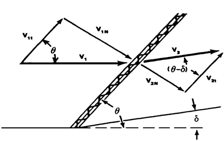
$$\delta = \text{surface turning angle}$$

$$\theta = \text{shock wave angle}$$

$$\text{Subscript 1 denotes upstream conditions}$$

$$\text{Subscript 2 denotes downstream conditions}$$

Oblique Shock Relations

• Calculate $P_2/P_1$, $T_2/T_1$, and $\rho_2/\rho_1$ across oblique shocks by using normal shock equations and substituting $M_1 \sin\theta$ in place of $M_1$
• Calculate total pressure loss across oblique shock as

$$\frac{P_{T_2}}{P_{T_1}} = \left[\left[\frac{\gamma - 1}{\gamma + 1} + \frac{2}{{\left(\gamma + 1\right)M_1^2\sin^2\theta}}\right]^{\gamma} \left[\frac{2\gamma}{\gamma+1} M_1^2\sin^2\theta - \frac{\gamma - 1}{\gamma + 1} \right]\right]^{\frac{1}{1 - \gamma}}$$

• Calculate relation between Mach number and angles as

$$M_2^2\sin^2\left(\delta - \theta\right) = \frac{M_1^2 \sin^2\theta + \frac{2}{\gamma-1}}{\frac{2\gamma}{\gamma - 1} M_1^2\sin^2\theta - 1}$$

Oblique Shock Turning Angle as a Function of Wave Angle

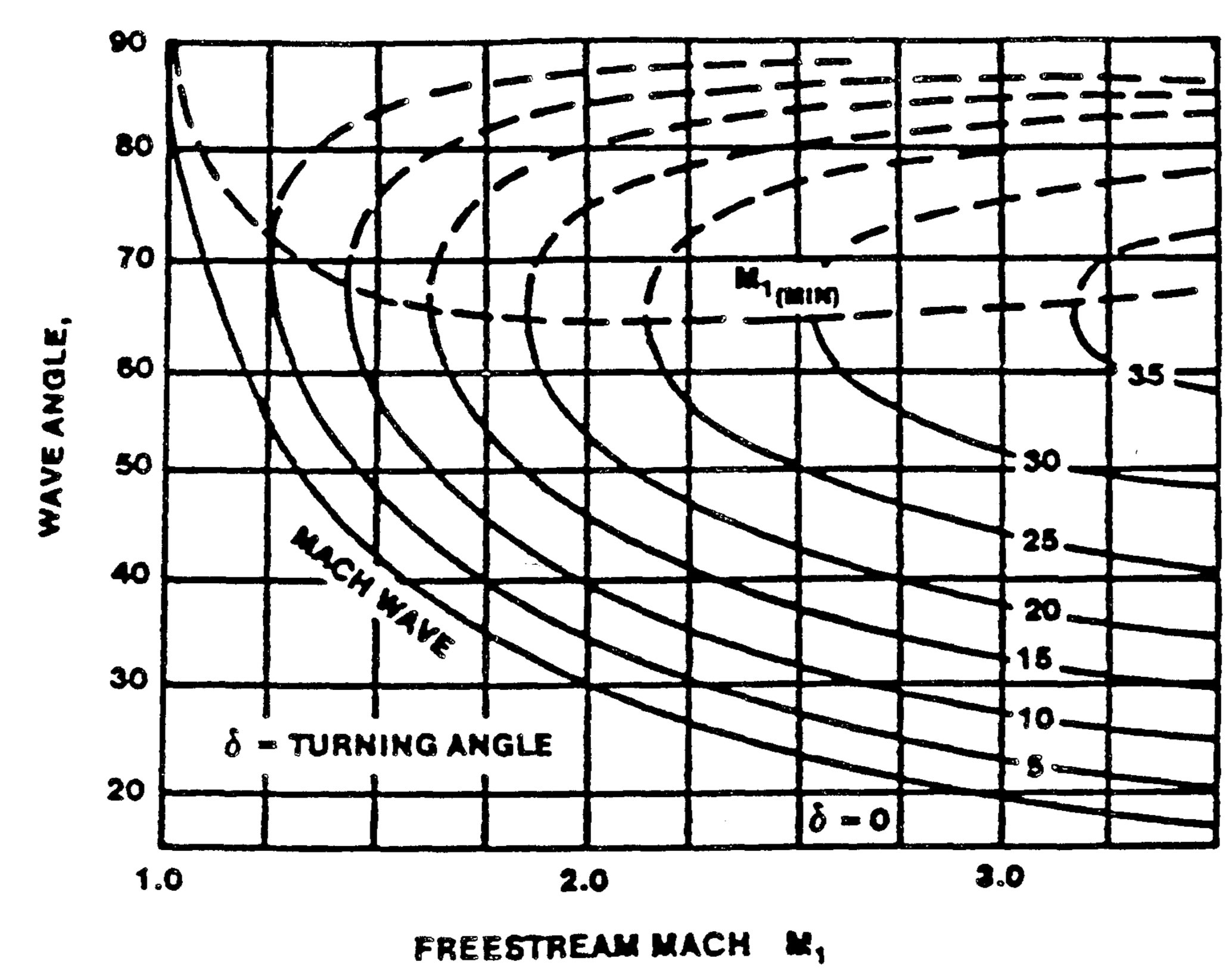
• Two $\theta$ solutions exist for every $M_1$ & $\delta$ combination
  • These represent the strong and weak shock solutions
  • Weak shocks normally occur in nature
• There is a minimum Mach number for each turning angle
• The wave angle of a weak shock decreases with increased Mach
• For a given Mach number, $\theta$ approaches $\mu$ as $\delta$ decreases

Mach Cone Angle

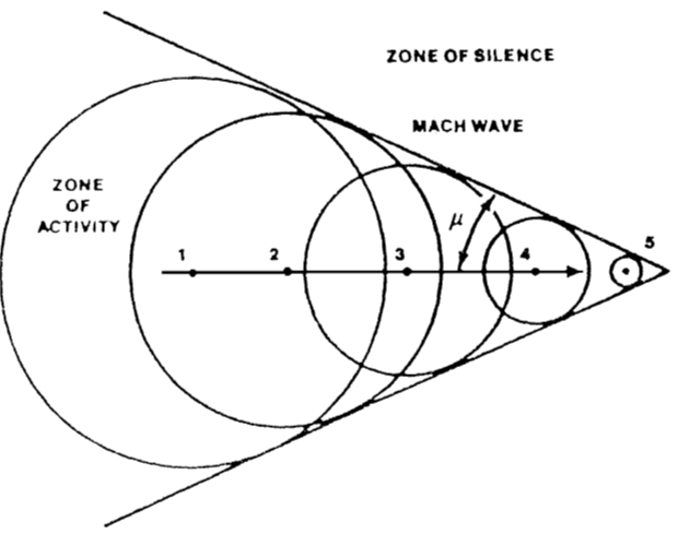
Minimum Wave Angle: $\mu = \sin^{-1}\left(1/M\right)$

5.5.2 Supersonic Isentropic Expansion Relation

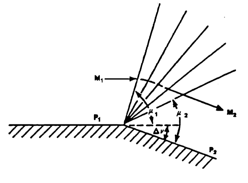
• The wave angle $\mu$ determines where the lower pressure can be felt and thus where the flow can be accelerated
• As the flow accelerates, a new wave angle forms and the subsequent lower pressure further accelerates the flow
• Results in a series of Mach waves forming a “fan” until the flow turns and accelerates so that it is parallel to the new boundary

Prandtl-Meyer Function

Shows flow’s required turning angle ($\nu$) to accelerate from one Mach number to another

$$\nu_M = \sqrt{\frac{\gamma + 1}{\gamma - 1}} \left[\tan^{-1}\sqrt{\frac{\gamma - 1}{\gamma + 1} \left(M^2 - 1\right)} \right] - \tan^{-1}\sqrt{M^2-1}$$

• If upstream Mach $(M_1) = 1$, then $\nu_1 = 0$, and equation directly relates downstream Mach ($M_2$) to surface turning angle ($\Delta \nu$)
• If $M_1 > 1$, determine $M_2$ as follows:
  • Calculate upstream ν₁ from above equation
  • Calculate $\nu_2 = \nu_1 + \Delta \nu$
  • Reverse above equation to obtain corresponding $M_2$
• Above equation is tabulated in NACA TR 1135 and is plotted below

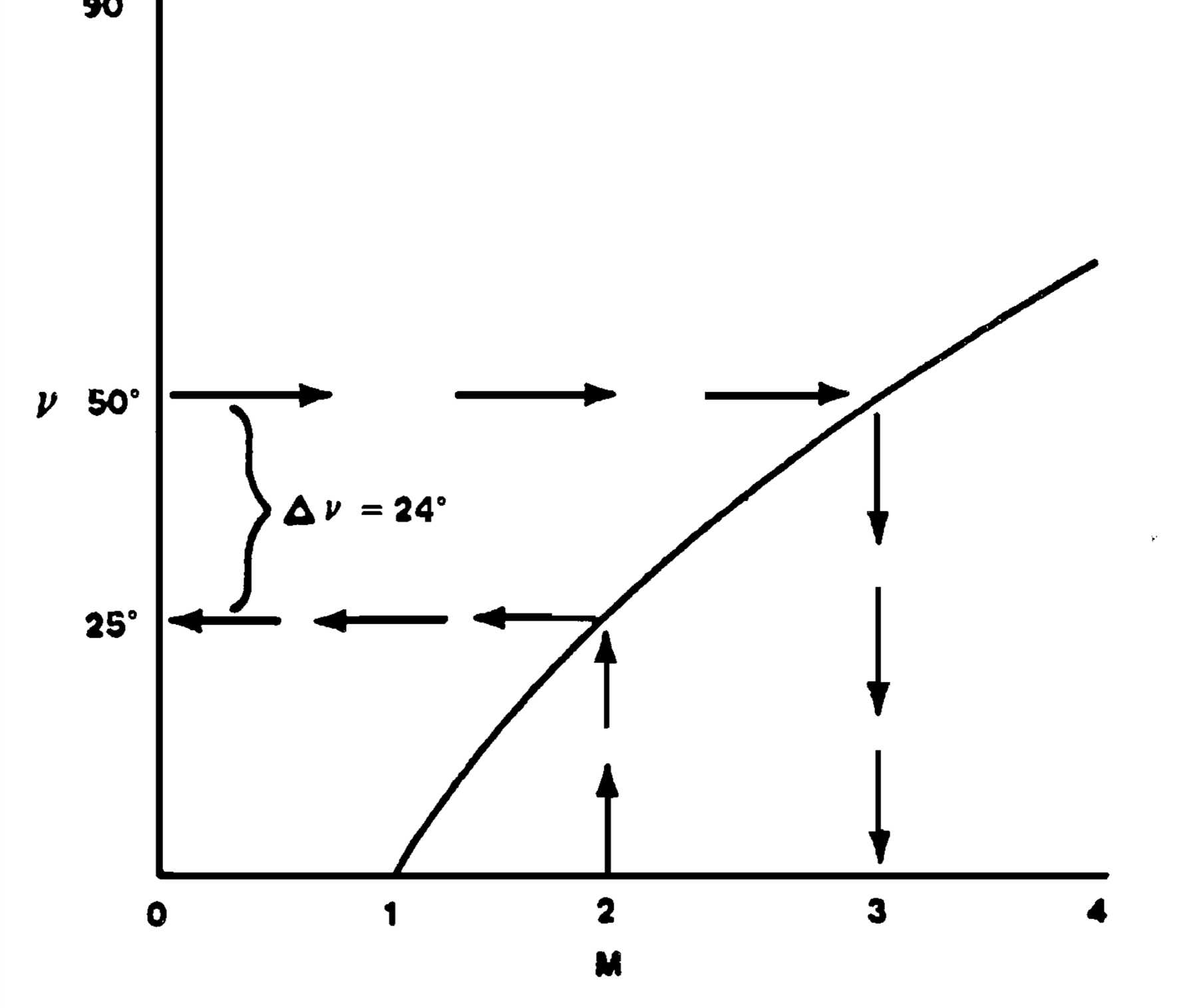
Example: Flow initially at $M_1 = 2.0$ accelerates through an expansion corner of 24 deg. Exit Mach number is 3.0

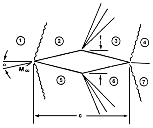
5.5.3 Two-Dimensional Supersonic Airfoil Approximations

• Determine surface static pressures by calculating changes through obliques shocks and expansion fans

• Ackert approximations for thin wings are based on

$$C_p = \frac{\Delta P}{q} \cong \pm\frac{2 \delta}{\sqrt{M^2 - 1}}$$

• Double wedge airfoil approximations

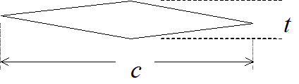
$$C_L \cong \frac{4 \alpha}{\sqrt{M^2 - 1} }$$

$$C_D \cong \frac{4 \alpha^2}{\sqrt{M^2 - 1}} + \frac{4}{\sqrt{M^2 - 1}}\left(\frac{t}{c}\right)^2$$

• Biconvex wing approximations

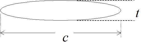
$$C_L \cong \frac{4 \alpha}{\sqrt{M^2 - 1} }$$

$$C_D \cong \frac{4 \alpha^2}{\sqrt{M^2 - 1}} + \frac{5.33}{\sqrt{M^2 - 1}}\left(\frac{t}{c}\right)^2$$

5.6 Drag Polars

(ref 5.2)

5.6.1 Drag Polar Construction and Terminology

$C_L = \text{lift coefficient}$

$C_D = \text{drag coefficient}$

$C_{D_i} = \text{induced drag coefficient}$

$C_{D_0} = \text{parasitic drag coefficient}$

$\mathrm{AR} = \text{aspect ratio}$

$e = \text{Oswald efficiency factor}$

$l = \text{length flow has traveled}$

$S_{\mathrm{wet}} = \text{wetted area of surface}$

$S = \text{reference wing area}$

Simple Drag Polar Equation Limitations

• No separated flow losses
• Symmetric Camber
• Applies at one Mach, Altitude, $\mathrm{cg}$

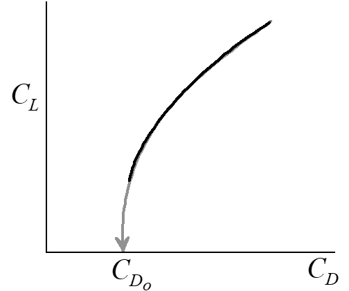
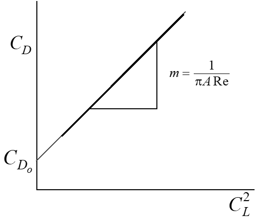
$$C_D = C_{D_0} + \frac{C_L^2}{\pi \mathrm{AR} e} = C_{D_0} + C_{D_i}$$

“Polar” form of simple drag polar:

Linearized form of simple drag polar:

5.6.2 Complicating Factors

Airflow Separation Effects

Drag Polar Equation Accounting for Flow Separation:

$$C_D = C_{D_{\mathrm{min}}} + \frac{\left(C_L - C_{L_{\mathrm{min}}}\right)^2}{\pi \mathrm{AR} e} +k_2\left(C_L - C_{L_{\mathrm{break}}}\right)$$

• Delete last term if $C_L < C_{L_{\mathrm{break}}}$
• Determine $k_2$ from flight test

Reynolds Number Effects

(refs 5.4, 5.11)

• Calculate length $\mathrm{Re}_L$ and friction coefficient ($c_f$) for each surface as

$$\mathrm{Re}_L = \frac{\rho Vl}{\mu} = 7.101 \times10^6 \left[\frac{\delta}{\theta^2} \right]\left[\frac{T_K + 110}{398}\right] l$$

$T_K = \text{Kelvin}$

$l = \text{total length, ft}$

$$c_f = \left[\frac{1.328}{\sqrt{\mathrm{Re}_L}}\right] \left[1 + 0.1305 M^2 \right]^{-0.12} \text{ laminar}$$ or $$c_f = \left[\frac{0.074}{\left(\mathrm{Re}_L\right)^2} - \frac{1700}{\mathrm{Re}_L} \right] \text{ transition}$$ or $$c_f = 0.455\left[\log \mathrm{Re}_L\right]^{-258} \left[1 + 0.144 M^2\right]^{-0.65} \text{ turbulent}$$

• In general, $c_f$ decreases as $\mathrm{Rn}$ increases (unless transitioning from laminar to turbulent flow)
• Friction drag $= c_f q S_{\mathrm{wet}}$ for each component ($S_{\mathrm{wet}} = \text{wetted area}$)
• Correct from test day to standard day aircraft drag coefficient by summing differences of each component’s drag change

$$\Delta C_D = \frac{\sum\left(c_{f_s} - c_{f_t} \right) S_{\mathrm{wet}}}{S}$$

Wing Camber or Incidence Angle Effects

Note slight increase in drag as lift decreases towards zero

Linearized drag polar for aircraft with wing camber and/or incidence

Revised drag polar equation accounting for wing camber or incidence

$$C_D = C_{D_{\mathrm{min}}} + \frac{\left(C_L - C_{L_{\mathrm{min}}} \right)^2}{\pi \mathrm{AR} e}$$

• Generally not necessary since most flight occurs above $C_{L_{\mathrm{min}}}$

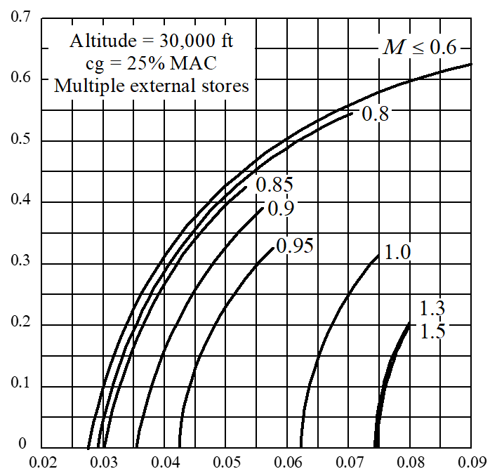
Mach Number Effects

• Aircraft with low parasitic drag coefficients and high fineness ratios pay a relatively small “wave drag” penalty.

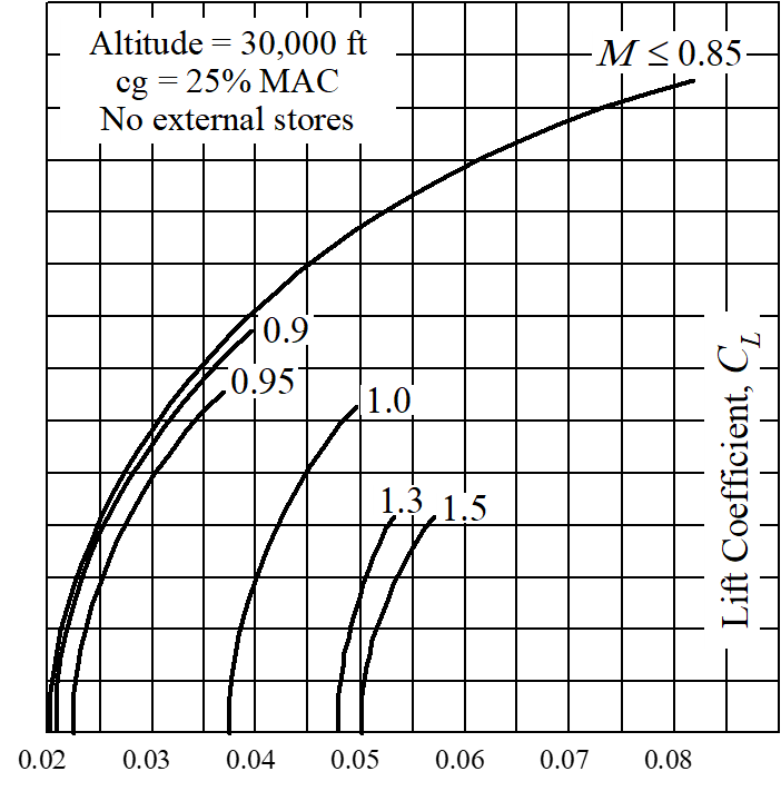
• With external stores, same aircraft pays larger Mach penalty

Propeller Slipstream Effects

• a.k.a “scrubbing” drag
• Propwash increases flow speed over surface within slipstream
• More drag is created by higher $q$ and vorticity.
• Function of prop speed and power absorbed ($C_p$) or thrust ($C_T$)
• Problem should be addressed in airframe or propeller models

Trim Drag Effects

(ref 5.4)

$e = \text{wing Oswald efficiency factor}$

$e_t = \text{tail Oswald efficiency factor}$

$b = \text{span}$

$b_t = \text{tail span}$

$x = \text{wing ac-to-cg distance}$

$l = \text{wing ac to tail ac distance}$

$S = \text{Area}$

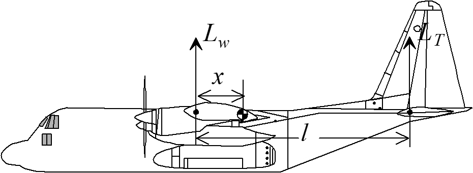
$$C_{D_{\mathrm{trim}}} = \frac{W^2}{\pi q^2 Sb^2e} \left[\frac{2}{lW}\left[x_0 - x_1\right] + \frac{1}{l^2} \left[1 + \frac{S}{S_t} \frac{e}{e_t} \left(\frac{b}{b_t}\right)^2\right] \left[x_0^2 - x_1^2\right] \right]$$

Trim drag change relative to total induced drag:

$$\frac{\Delta C_{D_{\mathrm{trim}}}}{\Delta C_{D_i}} = \frac{x}{l} \left[\frac{x}{l} \left(\frac{b}{b_t}\right)^2 \frac{e}{e_t} - 2 \right]$$

Plot of above equation

5.6.3 Drag Polar Analysis

$$D = \bar{q}SC_D = \bar{q}S \left[C_{D_0} + \frac{C_L^2}{\pi \mathrm{AR} e} \right] = \frac{1}{2}\rho_0 V_e^2 S\left[C_{D_0} + \frac{W^2}{\pi \mathrm{AR} e \left(\frac{1}{2} \rho_0 V_e^2 S \right)^2} \right]$$

• For a given configuration ($C_{D_0} \text{, } S \text{, } \mathrm{AR} \text{, } e$)

$$D = k_1 V_e^2 + k_2 \frac{W^2}{V_e^2}$$

first term = parasitic drag, second term = induced drag

• For any given weight, $D = f(\text{equivalent airspeed})$ only

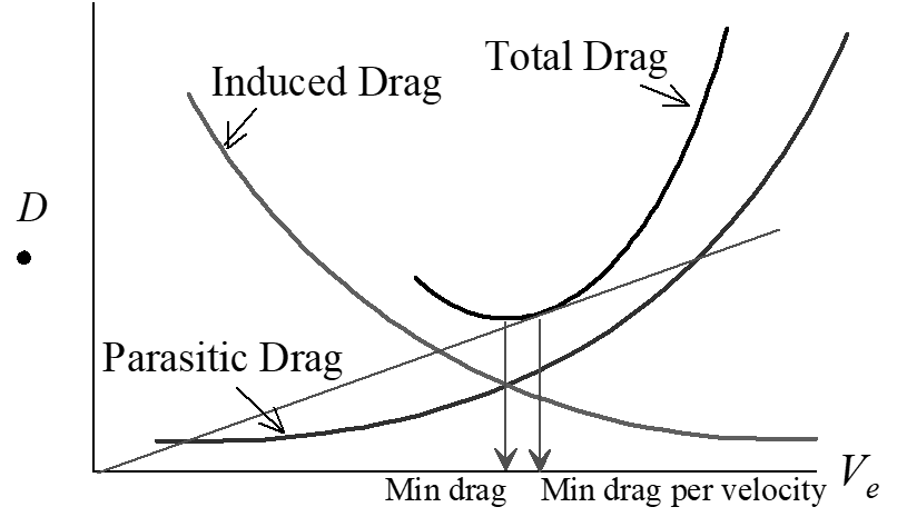
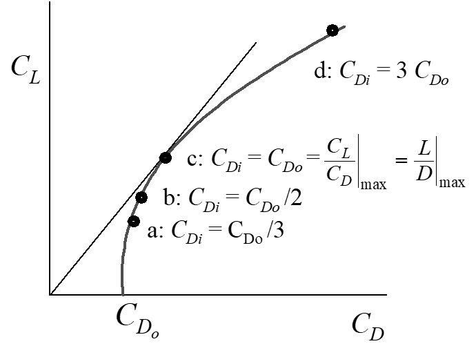
• Minimum total drag occurs when $D_{\mathrm{induced}} = D_{\mathrm{parasitic}}$
  • same as speed where $C_{D_i} = C_{D_0}$
  • occurs at max $C_L/C_D$ ratio (same as max $L/D$ ratio)
• Minimum drag/velocity occurs at min slope of Drag vs V curve
  • same as speed where $3C_{D_i} = C_{D_0}$
  • occurs at max $C_L^{1/2}/C_D$ ratio

Power required = drag x true airspeed

$$P_{\mathrm{req}} = DV_T = D\frac{V_e}{\sqrt{\sigma}} = k_1\frac{V_e^3}{\sqrt{\sigma}} + k_2\frac{W^2}{\sqrt{\sigma}V_e}$$

Minimum total $P_{\mathrm{req'd}}$ occurs when $P_{\mathrm{induced}} = P_{\mathrm{parasitic}}$

• same as speed where $C_{D_i} = 3C_{D_0}$
• occurs at max $C_L^{3/2}/C_D$ ratio

Minimum power/velocity occurs at min slope of $P_{\mathrm{req'd}}$ vs $V$ curve

• same as speed where $C_{D_i} = C_{D_0}$
• occurs at max $C_L /C_D$ ratio

Optimum Aerodynamic Flight Conditions

Gliders/ Engine-Out Flight

• Max range (minimum glide slope) occurs at max $C_L/C_D$
  • same as condition where $C_{D_0} = C_{D_i}$ if drag polar is parabolic
• Min sink rate (minimum power req’d) occurs at max $C_L^{3/2} /C_D$ ratio same as condition where $3C_{D_0} = C_{D_i}$ if drag polar is parabolic

Reciprocating Engine Aircraft (assuming constant $\mathrm{BSFC}$ & prop $\eta$)

• Max range (minimum power/velocity) occurs at max $C_L/C_D$ ratio
  • same as condition where $C_{D_0} = C_{D_i}$ if drag polar is parabolic
• Max endurance (minimum power req’d) occurs at max $C_L^{3/2} / C_D$
  • same as condition where $3C_{D_0} = C_{D_i}$ if drag polar is parabolic

Turbine Jet Engine Aircraft (assuming constant $\mathrm{TSFC}$)

• Max range at constant altitude (minimum drag/velocity)
  • occurs at max $C_L^{1/2} / C_D$ ratio
  • same as condition where $C_{D_0} = 3C_{D_i}$ if drag polar is parabolic
• Best cruise/climb range (maximum $\left[M \times L/D \right]$ ratio)
  • occurs at max $C_L/C_D^{3/2}$ ratio
  • same as condition where $C_{D_0} = 2C_{D_i}$ if drag polar is parabolic
• Best endurance (minimum drag)
  • occurs at max $C_L/C_D$ ratio
  • same as condition where $C_{D_0} = C_{D_i}$ if drag polar is parabolic

To calculate optimum speed $V_2$ for configuration₂ & weight₂ based on optimum speed $V_1$ at configuration₁ & weight₁

5.7 References

5.1	Roberts, Sean “Aerodynamics for Flight Testers” Chapter 3, Subsonic Aerodynamics, National Test Pilot School, Mojave, CA, 1999
5.2	Lawless, Alan R., et al, “Aerodynamics for Flight Testers” Chapter 4, Drag Polars, National Test Pilot School, Mojave ,CA, 1999
5.3	Hurt Hugh H., “Aerodynamics for Naval Aviators,” University of Southern California, Los Angeles, CA, 1959.
5.4	McCormick, Barnes W., “Aerodynamics, Aeronautics, and Flight Mechanics,” Wilet &Sons, 1979
5.5	Stinton, Darryl, “The Design of the Aeroplane,” BSP Professional Books, Oxford, 1983
5.6	Roskam, Jan Dr., “Airplane Design, Part VI,” Roskam Aviation and Engineering Corp. 1990
5.7	Anon, “Equations, Tables, and Charts for Compressible Flow” NACA Report 1135, 1953
5.8	Lewis, Gregory, “Aerodynamics for Flight Testers” Chapter 6, Supersonic Aerodynamics, National Test Pilot School, Mojave CA, 1999
5.9	White, Frank M. “Fluid Mechanics” pg 29, McGraw-Hill, 1979, ISBN 0-07-069667-5.
5.10	Anderson, John D. Jr, “Introduction to Flight” pg 142, McGraw-Hill, 1989, ISBN 0-07-001641-0.
5.11	Twaites, Bryan, Editor, “Incompressible Aerodynamics: An Account of the steady flow of incompressible Fluid Past Aerofoils, Wings, and Other Bodies,” Dover Publications, 1960.